


- Introduction
- Function Introduction
- Performance Monitor
- Fusion Hunter
- Quantitative Chart
- SEC Filing
- Insider Trading (Search by Ticker)
- Insider Trading (Search by Reporter)
- Insider Trading (Top Insider Trading)
- Institutional Holdings
- Investment Trends (Investment Company List)
- Investment Trends (Sector & Industry Sentiment)
- Investment Trends (Investment Company Sentiment)
- Investment Trends (Top Institutional Trading)
- Investment Trends (Top Institutional Hldg Change)
- Key Ratio Distribution
- Screener
- Financial Statement
- Key Metrics
- High Current Difference
- Low Current Difference
- Relative Strength Index
- KDJ
- Bollinger Bands
- Price Earnings Ratio
- Price to Book Value
- Debt Equity Ratio
- Leverage Ratio
- Return on Equity
- Return on Assets
- Gross Margin
- Net Profit Margin
- Operating Margin
- Income Growth
- Sales Growth
- Quick Ratio
- Current Ratio
- Interest Coverage
- Institutional Ownership
- Sector & Industry Classification
- Data Portal
- API
- SEC Forms
- Form 4
- Form 3
- Form 5
- CT ORDER
- Form 13F
- Form SC 13D
- Form SC 14D9
- Form SC 13G
- Form SC 13E1
- Form SC 13E3
- Form SC TO
- Form S-3D
- Form S-1
- Form F-1
- Form 8-k
- Form 1-E
- Form 144
- Form 20-F
- Form ARS
- Form 6-K
- Form 10-K
- Form 10-Q
- Form 10-KT
- Form 10-QT
- Form 11-K
- Form DEF 14A
- Form 10-D
- Form 13H
- Form 24F-2
- Form 15
- Form 25
- Form 40-F
- Form 424
- Form 425
- Form 8-A
- Form 8-M
- Form ADV-E
- Form ANNLRPT
- Form APP WD
- Form AW
- Form CB
- Form CORRESP
- Form DSTRBRPT
- Form EFFECT
- Form F-10
- Form F-3
- Form F-4
- Form F-6
- Form F-7
- Form F-9
- Form F-n
- Form X-17A-5
- Form F-X
- Form FWP
- Form G-405
- Form G-FIN
- Form MSD
- Form N-14
- Form N-18F1
- Form N-18F1
- Form N-30B-2
- Form N-54A
- Form N-8A
- Form N-CSR
- Form N-MFP
- Form N-PX
- Form N-Q
- Form TTW
- Form TA-1
- Form T-3
- Form SC 14F1
- Form SE
- Form SP 15D2
- Form SUPPL
- Form 10-12G
- Form 18-K
- Form SD
- Form STOP ORDER
- Form TH
- Form 1
- Form 19B-4(e)
- Form 40-APP
- Form 497
- Form ABS-15G
- Form DRS
- Form MA
- Form UNDER
- AI sentiment
- Access guide
- Academy
- Term of service
- GDPR compliance
- Contact Us
- Question Center
| Font Size: |
Quantitative Chart
"Quantitative Chart" provides quick look up of daily/weekly stock price, technical/fundamental indicators, and quantitative predictions. The daily technical indicators and quantitative predictions in "Quantitative Chart" are updated daily around 19:30 CDT -- about 4.5 hours * after the end of core trading session of major US stock exchanges. The weekly indicators are updated every friday at about 19:40 CDT.
* The time is used for post processing including data cleaning, calibration, and statistical analysis. We are working hard to shorten the processing time, and will keep users updated on any improvement.
- Navigator Options
- Fundamental Briefing
- Major Support/Resistence Levels
- Price Variation
- Technical Charts
- Markov Chain Prediction
Navigator Options
-
Spt/Rst Region Definition
The percentage threshold to define support or resistance region. Take SMA20w (20-week simple moving average) for example, when this value is set to 2%, a daily high price located within 2% region below SMA20w will make SMA20w an effective resistance level. A daily low price located within 2% region above SMA20w will make SMA20w an effective support level.
-
Intra/Inter Day Cross
The number of trading days to trace back to calculate the possibility of crossover through each levels. This parameter is also used to determine the possibility of support/resistance for each levels.
Fundamental Briefing
This section provides weekly updated fundamental indicators as well as quantile rankings in corresponding industry, sector, and the whole US market. See Key Metrics for detailed definition of each indicator. Specifically, four indicators (i.e. price/earnings ratio, price to book value, price to sales, price to operating income) also have daily updated values (Shown in cyan color) after market close on each trading day.
Major Support/Resistence Levels
This section provides about 40 support/resistence levelsa to help investors optimize entry/exit point. We recommend to enter a long (or short) position in close vicinityb of support (or resistence) line, and exit (stop loss order) immediately once the stock price moves against your position and cross corresponding line. In practice, you may need to set stop loss price slightly below (or above) support (or resistence) line to allow for market volatility.
a The number of levels differs between stocks due to different data availability.
b The definition of "close vicinity" differs between investors due to different risk tolerance.
Here is brief explanation of the support/resistence levels
-
FR_TREND_PURE [(L/U) (90%/95%/99%)]: Time series regression using only trend factor as independent variable. FR_TREND_PURE represents the predicted stock price. 'L' and 'U' represents lower and upper boundary of (90%/95%/99%) confidence intervals, respectively.
-
FR_TREND_BASIC [(L/U) (90%/95%/99%)]: Fundamental regresssion with time series trend, using EPS, BPS, debt equity ratio, and trend factor as independent variable. FR_TREND_BASIC represents the predicted stock price. 'L' and 'U' represents lower and upper boundary of (90%/95%/99%) confidence intervals, respectively.
-
FR_TREND [(L/U) (90%/95%/99%)]: Fundamental regresssion with time series trend, using EPS, BPS, RPS, OEPS, debt equity ratio, operating cash flow, quick ratio, and trend factor as independent variable. FR_TREND represents the predicted stock price. 'L' and 'U' represents lower and upper boundary of (90%/95%/99%) confidence intervals, respectively.
-
52-week High/Low: The highest/lowest price in the past 52 weeks.
-
Pivot Point: previous (high + low + close)/3.
-
BB(20w/20d) Lower/Upper: The lower/upper boundary of 20-week/20-day Boll's Band.
-
SMA(50w/20w/10w/50d/20d/10d): The 50-week/20-week/10-week/50-day/20-day/10-day simple moving average.
Probability of crossover and support/resistance
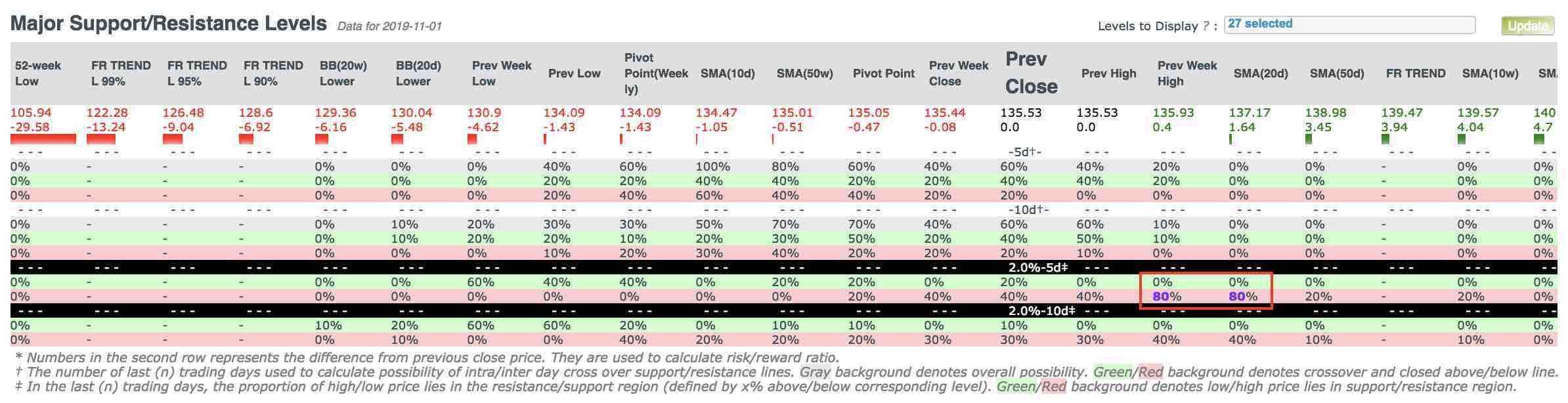
You can fine tune entry/exit point by relying on the probability chart as shown above. In this example, historical data from the past 5 trading days indicates "Prev Week High" and "SMA(20d)" functioned as resistance level 80% of the times (i.e. 4 trading days). Our experience is that long/short positions built around support/resistance levels with high probabilities are significantly more stable and not easily squeezed out in a volatile market.
Price Variation
This section provides price variation of previous trading day and upper 95%/99% confidence interval(CI) of 10-day/week price variation (i.e. (High - Low)/Close * 100%), shown in both percentage and dollar value. Specifically, a price variation exceeds upper 95% CI of 10-period price variation signals potential reversal, as shown below.
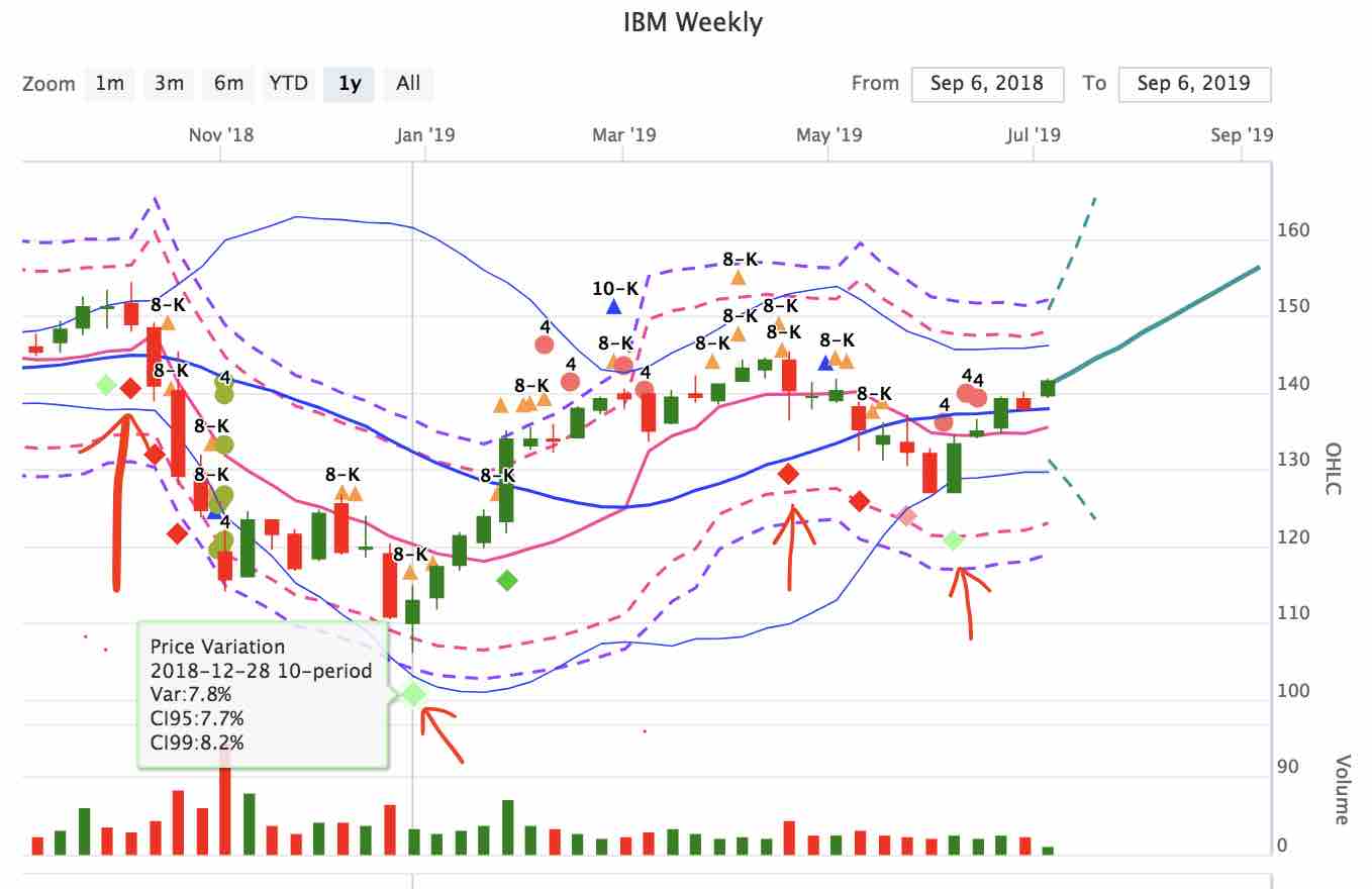
Analysis of weekly price movement of IBM indicates obvious reversal after significant price variation (marked by green or red diamond below candle bar) at 4 different time points.
The price variation data can also be helpful in setting trailing stop order. When price moves away from peak/valley for a significant amount, you should consider to take profit and exit.
Technical Charts
"Quantitative Chart" provides daily and weekly technical charts that are displayed simultaneously (either horizontally or vertically). You can display traditional technical indicators as well as overlay other kinds of information as shown below.
-
Fundamental Indicators Overlay
Simultaneously overlay up to 7 fundamental indicators like "Earnings Per Share","Book Value Per Share", "Revenue Per Share", "Net Profit Margin". There are more than 30 fundamental indicators available. Check respective sections of Key Metrics for detail. Fundamental indicators are updated weekly.
-
Quantitative Prediction Overlay
Overaly several quantitative analysis metrics that are proved to be more powerful than traditional technical indicators in many scenarios
FR/FR_TREND/FR_TREND_BASIC/FR_TREND_PURE: They are briefly introduced in the Major support/resistence levels. Here we give more details
Fundamental Regression (FR) Prediction
FR prediction includes regression line with 95% confidence interval (CI) and adjusted R-square value. The FR model is established per stock by using close price as dependent variable and 7 fundamental indicators as dependent variable (EPS, BPS, RPS, OEPS, debt equity ratio, operating cash flow, quick ratio, missing value not allowed). The model is built on weekly data from trailing 2 years, and a minimum of 60 weeks are required. A prediction is made based on the final model, with 95% CI and adjusted R-square been reported together.
FR is updated daily after market close, assuming close price of current trading day as weekly close price. The predictions (fitted value for the last observation) given by FR should be viewed as medium term target price.Fundamental Regression with Time Series Trend (FR_TREND) (recommended)
FR_TREND incorporates time trend as an independent variable into the regression model with fundamental indicators. Each time point is assigned an integar from 1 to the length of data. FR_TREND is better than FR in capturing short term momentum. In practice, we noticed plenty of evidence of stock prices dip or hike to near 95% or 99% confidence interval of FR_TREND, which are frequently far beyond the boundary of typical (20-period daily or weekly) Boll's upper or lower band. See example for Google below
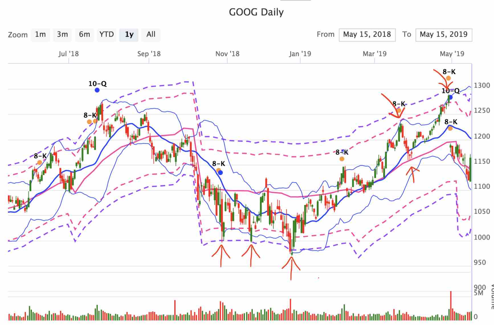
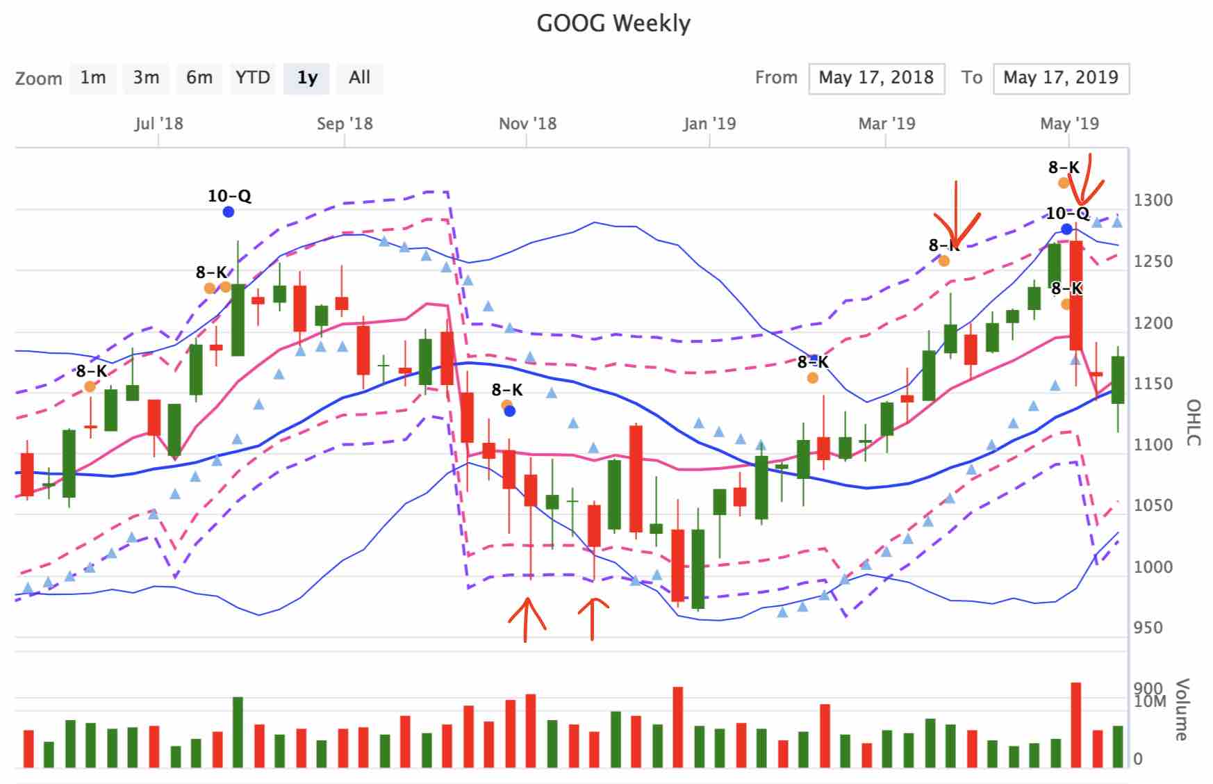
This greatly complements a major deficiency of Boll's band that there is no explicit stop or reversal point when price starts to move along the upper/lower boundary of Boll's band. In the example above, the range of price movement is apparently beyong the reach of BB's lower or upper boundary. Several reversal points are located almost exactly on 95% or 99% CI of FR_TREND line. Your stop loss strategies will doubtlessly be greatly improved with the assistance of FR_TREND.
FR_TREND is updated at the same time as FR.
Fundamental Regression BASIC (FR_TREND_BASIC)
This is simplified version of FR_TREND by including only EPS, BPS, debt equity ratio, and trend factor. Missing value not allowed
Fundamental Regression PURE (FR_TREND_PURE)
Only trend factor is used in regression model
ARIMA Prediction
ARIMA is abbreviation for auto regression integrated moving average, which is highly popular in the field of quantitative investment analysis. ARIMA is performed separately when predicting daily and weekly close price. For daily close price prediction, the model is built on historical daily close of trailing 1 year, and a minimum of 200 trading days are required. For weekly close price prediction, the model is built on historical weekly close of trailing 2 years, and a minimum of 40 weeks are required. The level of differencing (d), order of auto regression model (p), and order of moving average model (q) are determining through an automatic process which minimizes AIC.
ARIMA is performed daily after market close. The predictions given by ARIMA should be viewed as short term target price. It is noteworthy the the 95% CI given by ARIMA prediction is very helpful in determining the range of price movement for the upcoming day/week.ARIMA 10 periods forecast with 2-level differencing
The 2-level differencing of Y at period t is equal to (Yt - Yt-1) - (Yt-1 - Yt-2) = Yt - 2Yt-1 + Yt-2. It measures the "acceleration" or "curvature" in price movement at a given time point. It is generally equivalent to Holt's exponential smooth with trend, with the exception that ARIMA also captures autoregression components.
The 10 periods forecast should be understood as generally trend given currently observed close prices. The long term forecast should not be viewed as price target. -
SEC Filings Overlay
Overlay important SEC filings like "10-K" (annual report), "10-Q"(quarterly report), "8-K"(current report). We are expanding the list as necessary. SEC filings are shown as triangles with different colors. Click any triangle to open corresponding original filing in a new window. Follow SEC Forms in respective sections for detailed definition of each form type.
-
Insider Transactions Overlay
Insider transactions filed in Form 3/4/5 grouped by transaction types. There are 20 different types(codes) of transaction. Follow Form 4 for details of each transaction type.
-
Other Overlays
Dividend History: Includes both historical and upcoming dividends.
-
Chart Layout
Switch between vertical and horizontal display of daily and weekly chart.
-
Technical Indicators
Indicator Abbreviation Available Configuration(s) Open, High, Low, Close OHLC Daily, Weekly Bollinger Bands BB 20/2 Bollinger Bands Width BBW 20/2 Bollinger Bands %b BBP 20/2 Bollinger Bands Constrain BBC 10; 5 Commodity Channel Index CCI 20 Chaikin Money Flow CMI 9; 14; 20 Exponential Moving Average EMA 5; 10; 14; 20; 50; 100; 200 Ichimoku Cloud IKH 26/9/52 Stochastic Oscillator (Slow/Fast) KDJ (slow/fast) 9/3/3; 14/3/3; 20/3/3 Moving Average Convergence Divergence MACD 12/26/9 Money Flow Index MFI 9; 14; 20 Parabolic SAR PSAR 0.02/0.2 Relative Strength Index (Smoothed/Non-Smoothed) RSI 5; 9; 14; 20; 25 Simple Moving Average SMA 5; 10; 20; 50; 100; 200 Zigzag Zigzag 1%~10% Note that the technical indicators shown in the technical charts are calculated on the fly using the OHLC data, which are updated daily after market close. For weekly charts, this may generate premature weekly signal before the end of the last trading day of a week.
Markov Chain Prediction
Markov chains of various orders (1st order to 4th order, as well as mixed orders) are used to predict the weekly price movement direction, where UP(or DOWN) represents predicted weekly close (of the upcoming week) higher(or lower) than previous weekly close.
For each stock, up to 3 years (and no less than 60 weeks) historical weekly close prices were used to construct markov chain probability model, which is used to make prediction of upcoming weekly price movement based on observation(s) from previous week(s). The order of markov model represents the number of trailing weeks utilized to make prediction. See example results below
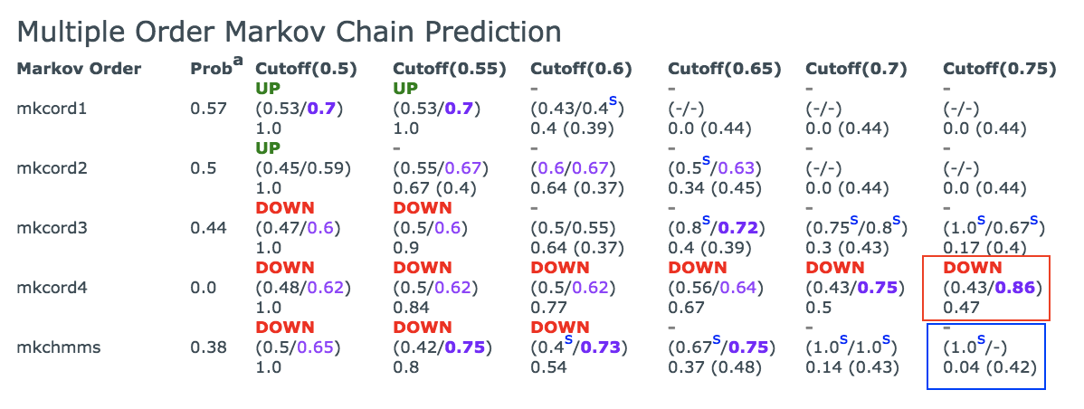
The first field ("Markov Order") shows the order of markov chain, where "mkcord1" represents 1st order, "mkcord2" represents 2nd order, and so on. "mkchmms" represents hidden markov states weighted markov chain, which will be discussed later. The second field ("Prob") shows the probability of observing an UP event according to corresponding markov chain. When the probability is higher than 0.5, there is a greater chance that the upcoming week will close higher than previous week (an UP prediction). When lower than 0.5, there is a greater chance that the upcoming week will close lower than previous week (a DOWN prediction). The rest of fields with cutoff values from 0.5 to 0.75 are used to set up a threshold for making prediction. For example, when the cutoff value is set to 0.75, we only make an UP (or DOWN) prediction when markov chain shows probability >=0.75 (or <= 1 - 0.75).
More importantly, we are more interested the precision (or Positive Predictive Value, PPV) of the predictions, which are calculated by comparing historically the predicted directions and actually observed directions of corresponding markov model at given cutoff value. The precisions are calculated separately for UP and DOWN predictions, as shown in the red rectangle above. In this example, the precision of DOWN prediction is 0.86, which means for the N trailing weeks (N <=50 and >=15) with weekly price movement >=1% (the 1% threshold is arbitrarily chosen to avoid random noise), 86% of the DOWN predictions were proved correct (and 14% were proved wrong). On the other hand, the precision of UP prediction is 0.43, which means the UP predictions made by the markov chain at the given cutoff threshold were correct 43% of the times (and 57% predictions were proved wrong).
The first number 0.47 on the third lines gives the overall coverage rate, which represents the proportion of times the markov model was able to make a prediction at the given cutoff value.
An additional number will be shown in parentheses next to coverage rate (see the blue rectangle) when a markov model can not make a prediction at given cutoff value. The number indicates the proportion of actually observed UP events when predictions can not be explicitly made.
Note that we are interested in precisions (or proportions) notably deviate from 0.5 (i.e. a precision equal to 0.8 is as same interesting as a precision equal to 0.2). For example, an UP prediction with 0.2 precision should be interpreted as a strong probability of DOWN, because the predictions are 80% wrong!
Mixed Order Markov Chain
Mixed Order Markov Chain makes prediction by taking average over probabilities from two markov chains. The other procedures are the same as above.
Hidden Markov States Weighted Markov Chain
Hidden markov model with four hidden states is fitted to percentage changes in weekly close prices as continuous variable. Each state emits observations according to univariate normal distribution with initial mean and variance determined by K-MEANS clustering. The optimal hidden states sequence is determined by Viterbi's algorithm. The hidden states were then used to calculate weighted markov chain probabilities (more weights are given to the observation sequences with hidden state same as the last hidden state in the sequence). The motivation is that price movement should follow historical patterns with hidden state more similar to current state.
The above procedures are performed for 1st to 4th order markov models. The "Prob" field of "mkchmms" represents the average probability over four markov models.